Atmospheric Pressure Testing of Manifold Pressure Sensor (MPS)

We know that the MPS changes the pulse width based on the manifold vacuum and the atmospheric pressure. Testing for the manifold vacuum is straightforward – attached a MityVac to the port on the back of the MPS and see what effect it has. Testing for atmospheric pressure is a little more difficult.

The MPS senses the atmospheric pressure through the center of the adjustment screw. Original Bosch factory caps have holes at the base of the cap to allow air to freely flow from the engine bay to the adjustment screw.

What we don’t know is how much of an effect the atmospheric pressure has on the injector pulses. This thread details my experimentation. The goal is to construct a set of formula or tables of data so we can take an MPS pulse width at atmospheric pressure X and correct it to sea level.

Why would we want to do that? It allows us to compare two MPSs directly that were measured at different altitudes and under different weather conditions.

For example if we have MPS A that has pulse widths measured at 900mb and MPS B that has pulse widths measured at 1000mb then we can correct both to sea level pressure (1013.25mb) and compare the pulse widths to see how far apart the tuning of A and B are.

So we need to know how injector pulse widths change if we take an MPS and move it from 900mb to 1013.25mb (keeping all other test conditions the same).

In order to change the atmospheric pressure of an MPS we need to place the adjustment screw into a pressure chamber. Here is what I came up with:

This is a 3D printed cylinder with one end open and 1.5″ o-ring installed in a channel. The 3D print has 4 perimeters and 60% infill, so denser than a typical 3D print would be. A 1/4″ barb to 1/8″ MIP is epoxied into the side and attached to 1/4″ tubing.

This pressure vessel is clamped over the MPS covering the adjustment screw.

I have a circuit board that can measure the pulse widths generated by the MPS and the atmospheric pressure using a highly accurate sensor, performing 20 measurements per second and sending them to a PC.

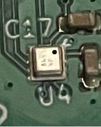
This sensor is 2mm x 2mm in size. It measures using the small black hole you can see on the top, however I don’t want to know what the pressure of the circuit board is, I want to know the pressure inside the chamber covering the adjustment screw. This means I need to loop it into the tubing.

Here is the solution I came up with.

This is a 1/4″ barb to 1/8″ FIP adapter with a compression nut. I epoxied them together and then I epoxied an o-ring to the bottom. I designed and printed a custom bracket to precisely position the o-ring over the top of the pressure sensor.

I didn’t expect this to work but actually it works really well. The tubing from the pressure sensor is then connected to the pressure chamber using a 1/4″ barb tee.

I still need to control the manifold vacuum but I only have one MityVac so I installed a ball valve (seen in the first picture in a different location) in the tube to the vacuum port. This allows me to first set the manifold vacuum, close the valve, disconnect the MityVac and attach it to the tubing to control the atmospheric pressure.

Here is a block diagram of the entire setup.

Orange = MPS, blue = air/pressure, green = electronics

The MityVac is connected to the ball valve OR the tee, depending on what I want to control.

The full setup:

One issue I had is that I am about 2,700ft above sea level, so if I only use the MityVac to reduce atmospheric pressure then I can only go up in elevation. I also needed to increase pressure to go down to sea level. My wife had the perfect idea – use a 20ml syringe – of which we have plenty from giving our dogs meds over the years.

After making 12,480 measurements here is the chart.

The bottom line is 0inHg of manifold vacuum and the top line is 15inHg, The lines in-between are increasing by 1inHg.

As you can see, nice linear relationships.

For reference 101,325Pa is sea level and 70,000Pa is roughly 10,000ft above sea level. This chart ranges from just below sea level to around 15,500ft.

Excel works out the slope of each line and from that I can calculate the percentage change in pulse width for each Pascal of pressure change.

Now we can work out a general formula:

PWt = PWm x (1 + ((PCPA x (PAt - PAm)) / 100))

PWm = measured pulse width (in ms)
PAm = measured pressure (in pascals)
PWt = pulse width at target pressure (in ms)
PAt = target pressure (in pascals)
PCPA = %/Pa from table above for desired manifold pressure

For example, we measure a pulse width of 16ms at an atmospheric pressure of 60,000Pa with a manifold vacuum of 0inHg. We want to know the pulse width for the same setup at sea level, 101,325Pa.

PAt – PAm = 101,325 – 60,000 = 41,325
PWm = 16
PCPA = 0.0000613029961957424000 (from the table)

Therefore PWt = 16 x (1 + ((0.0000613029961957424000 x 41325) / 100) = 16.4053ms

So fuel consumption is 2.5% higher at sea level than at ~13,800ft when the throttle is wide open.

Using this formula we can now compare two MPSs measured in different locations with different weather.

If we look at the chart we see a pattern – lots of straight lines. But there is a secondary pattern. As the pulse width and/or manifold vacuum increases the slope of the lines decrease. What is happening here?

So far I have kept the test conditions (engine speed and air temperature) the same and only varied the manifold pressure. What happens if we flip that around, keep the manifold pressure the same and vary the test conditions?

Here is a chart with the manifold vacuum kept at 0inHg but the test conditions were varied.

Note that there are two ways (other than atmospheric pressure) to change the injector pulse width:

– vary the manifold pressure
– vary the test conditions (engine speed and air temperature)

(in the full D-Jetronic system there are more inputs such as coolant temperature, but they are not part of any of this testing as they are applied by the ECU after the MPS has done it’s work, i.e. they don’t affect the MPS)

In this chart we can see the same pattern! As the pulse width increases the slope of the lines decreases. It seems that the slope of the lines is dependent on the pulse width (regardless of how that pulse width is changed). To put it another way we can change the pulse width via the manifold pressure or we can change the pulse width via the test conditions, but however we do it a longer pulse width equals a lower slope of the lines.

We can now create a new chart showing the relationship between pulse width and slope of the line.

his chart shows the relationship for three different manifold vacuum levels. The results do not appear to significantly vary based on the manifold vacuum, which confirms our suspicion that manifold vacuum is not affecting the slope of the lines.

Now we can take a pulse width and work out the line slope (which is the change in pulse width per Pascal). Here is the relationship (rearranged equation for blue line in previous chart):

LS = (PWm - 19.8823805648711) / -3.43310224625425 / 100000

PWm = measured pulse width (ms)
LS = line slope (ms/Pa)

We can now work out the pulse width for any atmospheric pressure (using any air temperature, manifold pressure and engine speed) as follows.

LS = (PWm - 19.8823805648711) / -3.43310224625425 / 100000
PAchange = PAt - PAm
PWchange = LS x PAchange
PWt = PWm + PWchange

Inputs:

PWm = measured pulse width (ms)
PAm = measured pressure (Pa)
PAt = target pressure (Pa)

Output:

PWt = pulse width at target pressure (ms)

If we set PAt to 101,325 then we will calculate the pulse width for sea level.

Conclusion: The MPS is an incredible piece of electro-mechanical engineering by Bendix/Bosch.

Download the pressure chamber STL. Print in PLA at 60% density with four shells.